Applied Statistics Lesson of the Day – The Full Factorial Design

An experimenter may seek to determine the causal relationships between factors and the response, where .  On first instinct, you may be tempted to conduct separate experiments, each using the completely randomized design with 1 factor.  Often, however, it is possible to conduct 1 experiment with  factors at the same time.  This is better than the first approach because

• it is faster
• it uses less resources to answer the same questions
• the interactions between the  factors can be examined

Such an experiment requires the full factorial design; in this design, the treatments are all possible combinations of all levels of all factors.  After controlling for confounding variables and choosing the appropriate range and number of levels of the factor, the different treatments are applied to the different groups, and data on the resulting responses are collected.  

The simplest full factorial experiment consists of 2 factors, each with 2 levels.  Such an experiment would result in  treatments, each being a combination of 1 level from the first factor and 1 level from the second factor.  Since this is a full factorial design, experimental units are independently assigned to all treatments.  The 2-factor ANOVA model is commonly used to analyze data from such designs.

In later lessons, I will discuss interactions and 2-factor ANOVA in more detail.

Applied Statistics Lesson of the Day – Choosing the Range of Levels for Quantitative Factors in Experimental Design

In addition to choosing the number of levels for a quantitative factor in designing an experiment, the experimenter must also choose the range of the levels of the factor.

• If the levels are too close together, then there may not be a noticeable difference in the corresponding responses.
• If the levels are too far apart, then an important trend in the causal relationship could be missed.

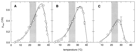
Consider the following example of making sourdough bread from Gänzle et al. (1998).  The experimenters sought to determine the relationship between temperature and the growth rates of 2 strains of bacteria and 1 strain of yeast, and they used mathematical models and experimental data to study this relationship.  The plots below show the results for Lactobacillus sanfranciscensis LTH2581 (Panel A) and LTH1729 (Panel B), and Candida milleri LTH H198 (Panel C).  The figures contain the predicted curves (solid and dashed lines) and the actual data (circles).  Notice that, for all 3 organisms,

• the relationship is relatively “flat” in the beginning, so choosing temperatures that are too close together at low temperatures (e.g. 1 and 2 degrees Celsius) would not yield noticeably different growth rates
• the overall relationship between growth rate and temperature is rather complicated, and choosing temperatures that are too far apart might miss important trends.

Once again, the experimenter’s prior knowledge and hypothesis can be very useful in making this decision.  In this case, the experimenters had the benefit of their mathematical models in guiding their hypothesis and choosing the range of temperatures for collecting the data on the growth rates.

Reference:

Gänzle, Michael G., Michaela Ehmann, and Walter P. Hammes. “Modeling of growth of Lactobacillus sanfranciscensis and Candida milleri in response to process parameters of sourdough fermentation.” Applied and environmental microbiology 64.7 (1998): 2616-2623.