How to Get the Frequency Table of a Categorical Variable as a Data Frame in R

Introduction

One feature that I like about R is the ability to access and manipulate the outputs of many functions.  For example, you can extract the kernel density estimates from density() and scale them to ensure that the resulting density integrates to 1 over its support set.

I recently needed to get a frequency table of a categorical variable in R, and I wanted the output as a data table that I can access and manipulate.  This is a fairly simple and common task in statistics and data analysis, so I thought that there must be a function in Base R that can easily generate this.  Sadly, I could not find such a function.  In this post, I will explain why the seemingly obvious table() function does not work, and I will demonstrate how the count() function in the ‘plyr’ package can achieve this goal.

The Example Data Set – mtcars

Let’s use the mtcars data set that is built into R as an example.  The categorical variable that I want to explore is “gear” – this denotes the number of forward gears in the car – so let’s view the first 6 observations of just the car model and the gear.  We can use the subset() function to restrict the data set to show just the row names and “gear”.

> head(subset(mtcars, select = 'gear'))
                     gear
Mazda RX4            4
Mazda RX4 Wag        4
Datsun 710           4
Hornet 4 Drive       3
Hornet Sportabout    3
Valiant              3

Mathematical and Applied Statistics Lesson of the Day – Don’t Use the Terms “Independent Variable” and “Dependent Variable” in Regression

In math and science, we learn the equation of a line as

,

with being called the dependent variable and being called the independent variable.  This terminology holds true for more complicated functions with multiple variables, such as in polynomial regression.

I highly discourage the use of “independent” and “dependent” in the context of statistics and regression, because these terms have other meanings in statistics.  In probability, 2 random variables and are independent if their joint distribution is simply a product of their marginal distributions, and they are dependent if otherwise.  Thus, the usage of “independent variable” for a regression model with 2 predictors becomes problematic if the model assumes that the predictors are random variables; a random effects model is an example with such an assumption.  An obvious question for such models is whether or not the independent variables are independent, which is a rather confusing question with 2 uses of the word “independent”.  A better way to phrase that question is whether or not the predictors are independent.

Thus, in a statistical regression model, I strongly encourage the use of the terms “response variable” or “target variable” (or just “response” and “target”) for and the terms “explanatory variables”, “predictor variables”, “predictors”, “covariates”, or “factors” for .

(I have encountered some statisticians who prefer to reserve “covariate” for continuous predictors and “factor” for categorical predictors.)

Applied Statistics Lesson of the Day – Notation for Fractional Factorial Designs

Fractional factorial designs use the notation; unfortunately, this notation is not clearly explained in most textbooks or web sites about experimental design.  I hope that my explanation below is useful.

• is the number of levels in each factor; note that the notation assumes that all factors have the same number of levels.
  • If a factor has 2 levels, then the levels are usually coded as and .
  • If a factor has 3 levels, then the levels are usually coded as , , and .
• is the number of factors in the experiment
• is the number of times that the full factorial design is fractionated by .  This number is badly explained by most textbooks and web sites that I have seen, because they simply say that is the fraction – this is confusing, because a fraction has a numerator and a denominator, and is just 1 number.  To clarify,
  • the fraction is
  • the number of treatments in the fractional factorial design is multiplied by the total possible number of treatments in the full factorial design, which is .

If all possible treatments are used in the experiment, then a full factorial design is used.  If a fractional factorial design is used instead, then denotes the fraction of the treatments that is used.

Most factorial experiments use binary factors (i.e. factors with 2 levels, ).  Thus,

• if , then the fraction of treatments that is used is .
• if , then the fraction of treatments that is used is .

This is why

• a design is often called a half-fraction design.
• a design is often called a quarter-fraction design.

However, most sources that I have read do not bother to mention that can be greater than 2; experiments with 3-level factors are less frequent but still common.  Thus, the terms half-fraction design and half-quarter design only apply to binary factors.  If , then

• a design uses one-third of all possible treatments.
• a design uses one-ninth of all possible treatments.

Applied Statistics Lesson of the Day – Fractional Factorial Design and the Sparsity-of-Effects Principle

Consider again an experiment that seeks to determine the causal relationships between  factors and the response, where .  Ideally, the sample size is large enough for a full factorial design to be used.  However, if the sample size is small and the number of possible treatments is large, then a fractional factorial design can be used instead.  Such a design assigns the experimental units to a select fraction of the treatments; these treatments are chosen carefully to investigate the most significant causal relationships, while leaving aside the insignificant ones.  

When, then, are the significant causal relationships?  According to the sparsity-of-effects principle, it is unlikely that complex, higher-order effects exist, and that the most important effects are the lower-order effects.  Thus, assign the experimental units so that main (1st-order) effects and the 2nd-order interaction effects can be investigated.  This may neglect the discovery of a few significant higher-order effects, but that is the compromise that a fractional factorial design makes when the sample size available is low and the number of possible treatments is high.  

Applied Statistics Lesson of the Day – Additive Models vs. Interaction Models in 2-Factor Experimental Designs

In a recent “Machine Learning Lesson of the Day“, I discussed the difference between a supervised learning model in machine learning and a regression model in statistics.  In that lesson, I mentioned that a statistical regression model usually consists of a systematic component and a random component.  Today’s lesson strictly concerns the systematic component.

An additive model is a statistical regression model in which the systematic component is the arithmetic sum of the individual effects of the predictors.  Consider the simple case of an experiment with 2 factors.  If is the response and and are the 2 predictors, then an additive linear model for the relationship between the response and the predictors is

In other words, the effect of on does not depend on the value of , and the effect of on does not depend on the value of .

In contrast, an interaction model is a statistical regression model in which the systematic component is not the arithmetic sum of the individual effects of the predictors.  In other words, the effect of on depends on the value of , or the effect of on depends on the value of .  Thus, such a regression model would have 3 effects on the response:

1. 
2. 
3. the interaction effect of and

A full factorial design with 2 factors uses the 2-factor ANOVA model, which is an example of an interaction model.  It assumes a linear relationship between the response and the above 3 effects.

Note that additive models and interaction models are not confined to experimental design; I have merely used experimental design to provide examples for these 2 types of models.

Applied Statistics Lesson of the Day – The Full Factorial Design

An experimenter may seek to determine the causal relationships between factors and the response, where .  On first instinct, you may be tempted to conduct separate experiments, each using the completely randomized design with 1 factor.  Often, however, it is possible to conduct 1 experiment with  factors at the same time.  This is better than the first approach because

• it is faster
• it uses less resources to answer the same questions
• the interactions between the  factors can be examined

Such an experiment requires the full factorial design; in this design, the treatments are all possible combinations of all levels of all factors.  After controlling for confounding variables and choosing the appropriate range and number of levels of the factor, the different treatments are applied to the different groups, and data on the resulting responses are collected.  

The simplest full factorial experiment consists of 2 factors, each with 2 levels.  Such an experiment would result in  treatments, each being a combination of 1 level from the first factor and 1 level from the second factor.  Since this is a full factorial design, experimental units are independently assigned to all treatments.  The 2-factor ANOVA model is commonly used to analyze data from such designs.

In later lessons, I will discuss interactions and 2-factor ANOVA in more detail.

Applied Statistics Lesson of the Day – The Matched Pairs Experimental Design

The matched pairs design is a special type of the randomized blocked design in experimental design.  It has only 2 treatment levels (i.e. there is 1 factor, and this factor is binary), and a blocking variable divides the experimental units into pairs.  Within each pair (i.e. each block), the experimental units are randomly assigned to the 2 treatment groups (e.g. by a coin flip).  The experimental units are divided into pairs such that homogeneity is maximized within each pair.

For example, a lab safety officer wants to compare the durability of nitrile and latex gloves for chemical experiments.  She wants to conduct an experiment with 30 nitrile gloves and 30 latex gloves to test her hypothesis.  She does her best to draw a random sample of 30 students in her university for her experiment, and they all perform the same organic synthesis using the same procedures to see which type of gloves lasts longer.

She could use a completely randomized design so that a random sample of 30 hands get the 30 nitrile gloves, and the other 30 hands get the 30 latex gloves.  However, since lab habits are unique to each person, this poses a confounding variable – durability can be affected by both the material and a student’s lab habits, and the lab safety officer only wants to study the effect of the material.  Thus, a randomized block design should be used instead so that each student acts as a blocking variable – 1 hand gets a nitrile glove, and 1 hand gets a latex glove.  Once the gloves have been given to the student, the type of glove is randomly assigned to each hand; some may get the nitrile glove on their left hand, and some may get it on their right hand.  Since this design involves one binary factor and blocks that divide the experimental units into pairs, this is a matched pairs design.

Applied Statistics Lesson of the Day – The Completely Randomized Design with 1 Factor

The simplest experimental design is the completely randomized design with 1 factor.  In this design, each experimental unit is randomly assigned to a factor level.  This design is most useful for a homogeneous population (one that does not have major differences between any sub-populations).  It is appealing because of its simplicity and flexibility – it can be used for a factor with any number of levels, and different treatments can have different sample sizes.  After controlling for confounding variables and choosing the appropriate range and number of levels of the factor, the different treatments are applied to the different groups, and data on the resulting responses are collected.  The means of the response variable in the different groups are compared; if there are significant differences, then there is evidence to suggest that the factor and the response have a causal relationship.  The single-factor analysis of variance (ANOVA) model is most commonly used to analyze the data in such an experiment, but it does assume that the data in each group have a normal distribution, and that all groups have equal variance.  The Kruskal-Wallis test is a non-parametric alternative to ANOVA in analyzing data from single-factor completely randomized experiments.

If the factor has 2 levels, you may think that an independent 2-sample t-test with equal variance can also be used to analyze the data.  This is true, but the square of the t-test statistic in this case is just the F-test statistic in a single-factor ANOVA with 2 groups.  Thus, the results of these 2 tests are the same.  ANOVA generalizes the independent 2-sample t-test with equal variance to more than 2 groups.

Some textbooks state that “random assignment” means random assignment of experimental units to treatments, whereas other textbooks state that it means random assignment of treatments to experimental units.  I don’t think that there is any difference between these 2 definitions, but I welcome your thoughts in the comments.

Applied Statistics Lesson of the Day – Choosing the Range of Levels for Quantitative Factors in Experimental Design

In addition to choosing the number of levels for a quantitative factor in designing an experiment, the experimenter must also choose the range of the levels of the factor.

• If the levels are too close together, then there may not be a noticeable difference in the corresponding responses.
• If the levels are too far apart, then an important trend in the causal relationship could be missed.

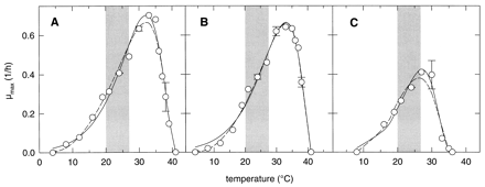
Consider the following example of making sourdough bread from Gänzle et al. (1998).  The experimenters sought to determine the relationship between temperature and the growth rates of 2 strains of bacteria and 1 strain of yeast, and they used mathematical models and experimental data to study this relationship.  The plots below show the results for Lactobacillus sanfranciscensis LTH2581 (Panel A) and LTH1729 (Panel B), and Candida milleri LTH H198 (Panel C).  The figures contain the predicted curves (solid and dashed lines) and the actual data (circles).  Notice that, for all 3 organisms,

• the relationship is relatively “flat” in the beginning, so choosing temperatures that are too close together at low temperatures (e.g. 1 and 2 degrees Celsius) would not yield noticeably different growth rates
• the overall relationship between growth rate and temperature is rather complicated, and choosing temperatures that are too far apart might miss important trends.

Once again, the experimenter’s prior knowledge and hypothesis can be very useful in making this decision.  In this case, the experimenters had the benefit of their mathematical models in guiding their hypothesis and choosing the range of temperatures for collecting the data on the growth rates.

Reference:

Gänzle, Michael G., Michaela Ehmann, and Walter P. Hammes. “Modeling of growth of Lactobacillus sanfranciscensis and Candida milleri in response to process parameters of sourdough fermentation.” Applied and environmental microbiology 64.7 (1998): 2616-2623.

Applied Statistics Lesson of the Day – Choosing the Number of Levels for Factors in Experimental Design

The experimenter needs to decide the number of levels for each factor in an experiment.

• For a qualitative (categorical) factor, the number of levels may simply be the number of categories for that factor.  However, because of cost constraints, an experimenter may choose to drop a certain category.  Based on the experimenter’s prior knowledge or hypothesis, the category with the least potential for showing a cause-and-effect relationship between the factor and the response should be dropped.
• For a quantitative (numeric) factor, the number of levels should reflect the cause-and-effect relationship between the factor and the response.  Again, the experimenter’s prior knowledge or hypothesis is valuable in making this decision.
  • If the relationship in the chosen range of the factor is hypothesized to be roughly linear, then 2 levels (perhaps the minimum and the maximum) should be sufficient.
  • If the relationship in the chosen range of the factor is hypothesized to be roughly quadratic, then 3 levels would be useful.  Often, 3 levels are enough.
  • If the relationship in the chosen range of the factor is hypothesized to be more complicated than a quadratic relationship, consider using 4 or more levels.

Applied Statistics Lesson of the Day – Basic Terminology in Experimental Design #1

The word “experiment” can mean many different things in various contexts.  In science and statistics, it has a very particular and subtle definition, one that is not immediately familiar to many people who work outside of the field of experimental design. This is the first of a series of blog posts to clarify what an experiment is, how it is conducted, and why it is so central to science and statistics.

Experiment: A procedure to determine the causal relationship between 2 variables – an explanatory variable and a response variable.  The value of the explanatory variable is changed, and the value of the response variable is observed for each value of the explantory variable.

• An experiment can have 2 or more explanatory variables and 2 or more response variables.
• In my experience, I find that most experiments have 1 response variable, but many experiments have 2 or more explanatory variables.  The interactions between the multiple explanatory variables are often of interest.
• All other variables are held constant in this process to avoid confounding.

Explanatory Variable or Factor: The variable whose values are set by the experimenter.  This variable is the cause in the hypothesis.  (*Many people call this the independent variable.  I discourage this usage, because “independent” means something very different in statistics.)

Response Variable: The variable whose values are observed by the experimenter as the explanatory variable’s value is changed.  This variable is the effect in the hypothesis.  (*Many people call this the dependent variable.  Further to my previous point about “independent variables”, dependence means something very different in statistics, and I discourage using this usage.)

Factor Level: Each possible value of the factor (explanatory variable).  A factor must have at least 2 levels.

Treatment: Each possible combination of factor levels.

• If the experiment has only 1 explanatory variable, then each treatment is simply each factor level.
• If the experiment has 2 explanatory variables, X and Y, then each treatment is a combination of 1 factor level from X and 1 factor level from Y.  Such combining of factor levels generalizes to experiments with more than 2 explanatory variables.

Experimental Unit: The object on which a treatment is applied.  This can be anything – person, group of people, animal, plant, chemical, guitar, baseball, etc.