Video Tutorial: Naive Bayes Classifiers

Naive Bayes classifiers are simple but powerful tools for classification in statistics and machine learning.  In this video tutorial, I use a simulated data set and illustrate the mathematical details of how this technique works.

In my recent episode on The Central Equilibrium about word embeddings and text classification, Mandy Gu used naive Bayes classifiers to determine if a sentence is toxic or non-toxic – a very common objective when moderating discussions in online forums.  If you are not familiar with naive Bayes classifiers, then I encourage you to watch this video first before watching Mandy’s episode on The Central Equilibrium.

Mandy Gu on Word Embeddings and Text Classification – The Central Equilibrium – Episode 9

I am so grateful to Mandy Gu for being a guest on The Central Equilibrium to talk about word embeddings and text classification.  She began by showing how data from text can be encoded in vectors and matrices, and then she used a naive Bayes classifier to classify sentences as toxic or non-toxic – a very common problem for moderating discussions in online forums.  I learned a lot from her in this episode, and you can learn more from Mandy on her Medium blog.

If you are not familiar with naive Bayes classifiers, then I encourage you to watch my video tutorial about this topic first.

Some SAS procedures (like PROC REG, GLM, ANOVA, SQL, and IML) end with “QUIT;”, not “RUN;”

Most SAS procedures require the

RUN;

statement to signal their termination.  However, there are some notable exceptions to this.

I have written about PROC SQL many times on my blog, and this procedure requires the

QUIT;

statement instead.

It turns out that there is another set of statistical procedures that require the QUIT statement, and some of them are very common.  They are called interactive procedures, and they include PROC REG, PROC GLM, and PROC ANOVA.  If you end them with RUN rather than QUIT, then you will run into problems with displaying further output.  For example, if you try to output a data set from one such PROC and end it with the RUN statement, then you will get this error message:

ERROR: You cannot open WORK.MYDATA.DATA for input access with record-level 
control because WORK.MYDATA.DATA is in use by you in resource environment 
REG.

WORK.MYDATA cannot be opened.

You will also notice that the Program Editor says “PROC … running” in its banner when you end such a PROC with RUN rather than QUIT.

I don’t like this exception, but, alas, it does exist.  You can find out more about these interactive procedures in SAS Usage Note #37105.  As this note says, the ANOVA, ARIMA, CATMOD, FACTEX, GLM, MODEL, OPTEX, PLAN, and REG procedures are interactive procedures, and they all require the QUIT statement for termination.

PROC IML is not mentioned in that usage note, but this procedure also requires the QUIT statement.  Rick Wicklin has written an article about this on his blog, The DO Loop.

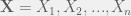
Arnab Chakraborty on The Monty Hall Problem and Bayes’ Theorem – The Central Equilibrium – Episode 6

I am pleased to welcome Arnab Chakraborty back to my talk show, “The Central Equilibrium“, to talk about the Monty Hall Problem and Bayes’ theorem.  In this episode, he shows 2 solutions to this classic puzzle in probability, and invokes Bayes’ Theorem for the second solution.

If you have not watched Arnab’s first episode on Bayes’ theorem, then I encourage you to do that first.

Marilyn Vos Savant provided a solution to this problem in PARADE Magazine in 1990-1991.  Thousands of readers disagreed with her solution and criticized her vehemently (and incorrectly) for her error.  Some of these critics were mathematicians!  She included some of those replies and provided alternative perspectives that led to the same conclusion.  Although I am dismayed by the disrespect that some people showed in their letters to her, I am glad that a magazine column on probability was able to attract so much readership and interest.  Arnab and I referred to one of her solutions in our episode.  Thank you, Marilyn!

Enjoy this episode of “The Central Equilibrium“!

Layne Newhouse on representing neural networks – The Central Equilibrium – Episode 4

I am excited to present the first of a multi-episode series on neural networks on my talk show, “The Central Equilibrium”.  My guest in this series in Layne Newhouse, and he talked about how to represent neural networks. We talked about the biological motivations behind neural networks, how to represent them in diagrams and mathematical equations, and a few of the common activation functions for neural networks.

Check it out!

A macro to execute PROC TTEST for multiple binary grouping variables in SAS (and sorting t-test statistics by their absolute values)

In SAS, you can perform PROC TTEST for multiple numeric variables in the same procedure.  Here is an example using the built-in data set SASHELP.BASEBALL; I will compare the number of at-bats and number of walks between the American League and the National League.

proc ttest
     data = sashelp.baseball;
     class League;
     var nAtBat nBB; 
     ods select ttests;
run;

Here are the resulting tables.

Method	Variances	DF	t Value	Pr > |t|
Pooled	Equal	320	2.05	0.0410
Satterthwaite	Unequal	313.66	2.06	0.04

Method	Variances	DF	t Value	Pr > |t|
Pooled	Equal	320	0.85	0.3940
Satterthwaite	Unequal	319.53	0.86	0.3884

 

What if you want to perform PROC TTEST for multiple grouping (a.k.a. classification) variables?  You cannot put more than one variable in the CLASS statement, so you would have to run PROC TTEST separately for each binary grouping variable.  If you do put LEAGUE and DIVISION in the same CLASS statement, here is the resulting log.

1303 proc ttest
1304 data = sashelp.baseball;
1305 class league division;
 --------
 22
 202
ERROR 22-322: Expecting ;.
ERROR 202-322: The option or parameter is not recognized and will be ignored.
1306 var natbat;
1307 ods select ttests;
1308 run;

 

There is no syntax in PROC TTEST to use multiple grouping variables at the same time, so this tutorial provides a macro to do so.  There are several nice features about my macro:

1. It allows you to use multiple grouping variables at the same time.
2. It sorts the t-test statistics by their absolute values within each grouping variable.
3. It shows the name of each continuous variable in the output table, unlike the above output.

Here is its basic skeleton.

A macro to automate the creation of indicator variables in SAS

In a recent blog post, I introduced an easy and efficient way to create indicator variables from categorical variables in SAS.  This method pretends to run logistic regression, but it really is using PROC LOGISTIC to get the design matrix based on dummy-variable coding.  I shared SAS code for how to do so, step-by-step.

I write this follow-up post to provide a macro that you can use to execute all of those steps in one line.  If you have not read my previous post on this topic, then I strongly encourage you to do that first.  Don’t use this macro blindly.

Here is the macro.  The key steps are

1. Run PROC LOGISTIC to get the design matrix (which has the indicator variables)
2. Merge the original data with the newly created indicator variables
3. Delete the “INDICATORS” data set, which was created in an intermediate step

%macro create_indicators(input_data, target, covariates, output_data);

proc logistic
     data = &input_data
          noprint
          outdesign = indicators;
     class &covariates / param = glm;
     model &target = &covariates;
run;


data &output_data;
      merge    &input_data
               indicators (drop = Intercept &target);
run;


proc datasets 
     library = work
          noprint;
     delete indicators;
run;

%mend;

I will use the built-in data set SASHELP.CARS to illustrate the use of my macro.  As you can see, my macro can accept multiple categorical variables as inputs for creating indicator variables.  I will do that here for the variables TYPE, MAKE, and ORIGIN.

An easy and efficient way to create indicator variables (a.k.a. dummy variables) from a categorical variable in SAS

Introduction

In statistics and biostatistics, the creation of binary indicators is a very useful practice.

• They can be useful predictor variables in statistical models.
• They can reduce the amount of memory required to store the data set.
• They can treat a categorical covariate as a continuous covariate in regression, which has certain mathematical conveniences.

However, the creation of indicator variables can be a long, tedious, and error-prone process.  This is especially true if there are many categorical variables, or if a categorical variable has many categories.  In this tutorial, I will show an easy and efficient way to create indicator variables in SAS.  I learned this technique from SAS usage note #23217: Saving the coded design matrix of a model to a data set.

The Example Data Set

Let’s consider the PRDSAL2 data set that is built into the SASHELP library.  Here are the first 5 observations; due to a width constraint, I will show the first 5 columns and the last 6 columns separately.  (I encourage you to view this data set using PROC PRINT in SAS by yourself.)

COUNTRY	STATE	COUNTY	ACTUAL	PREDICT
U.S.A.	California		$987.36	$692.24
U.S.A.	California		$1,782.96	$568.48
U.S.A.	California		$32.64	$16.32
U.S.A.	California		$1,825.12	$756.16
U.S.A.	California		$750.72	$723.52

 

PRODTYPE	PRODUCT	YEAR	QUARTER	MONTH	MONYR
FURNITURE	SOFA	1995	1	Jan	JAN95
FURNITURE	SOFA	1995	1	Feb	FEB95
FURNITURE	SOFA	1995	1	Mar	MAR95
FURNITURE	SOFA	1995	2	Apr	APR95
FURNITURE	SOFA	1995	2	May	MAY95

Video Tutorial – Obtaining the Expected Value of the Exponential Distribution Using the Moment Generating Function

In this video tutorial on YouTube, I use the exponential distribution’s moment generating function (MGF) to obtain the expected value of this distribution.  Visit my YouTube channel to watch more video tutorials!

Video Tutorial – The Moment Generating Function of the Exponential Distribution

In this video tutorial on YouTube, I derive the moment generating function (MGF) of the exponential distribution.  Visit my YouTube channel to watch more video tutorials!

Arnab Chakraborty on Bayes’ Theorem – The Central Equilibrium – Episode 3

Arnab Chakraborty kindly came to my new talk show, “The Central Equilibrium”, to talk about Bayes’ theorem.  He introduced the concept of conditional probability, stated Bayes’ theorem in its simple and general forms, and showed an example of how to use it in a calculation.

Check it out!

Christopher Salahub on Markov Chains – The Central Equilibrium – Episode 2

It was a great pleasure to talk to Christopher Salahub about Markov chains in the second episode of my new talk show, The Central Equilibrium!  Chris graduated from the University of Waterloo with a Bachelor of Mathematics degree in statistics.  He just finished an internship in data development at Environics Analytics, and he is starting a Master’s program in statistics at ETH Zurich in Switzerland.

Chris recommends “Introduction to Probability Models” by Sheldon Ross to learn more about probability theory and Markov chains.

The Central Equilibrium is my new talk show about math, science, and economics. It focuses on technical topics that involve explanations with formulas, equations, graphs, and diagrams.  Stay tuned for more episodes in the coming weeks!

You can watch all of my videos on my YouTube channel!

Please watch the video on this blog.  You can also watch it directly on YouTube.

Store multiple strings of text as a macro variable in SAS with PROC SQL and the INTO statement

I often need to work with many variables at a time in SAS, but I don’t like to type all of their names manually – not only is it messy to read, it also induces errors in transcription, even when copying and pasting.  I recently learned of an elegant and efficient way to store multiple variable names into a macro variable that overcomes those problems.  This technique uses the INTO statement in PROC SQL.

To illustrate how this storage method can be applied in a practical context, suppose that we want to determine the factors that contribute to a baseball player’s salary in the built-in SASHELP.BASEBALL data set.  I will consider all continuous variables other than “Salary” and “logSalary”, but I don’t want to write them explicitly in any programming statements.  To do this, I first obtain the variable names and types of a data set using PROC CONTENTS.

* create a data set of the variable names;
proc contents
     data = sashelp.baseball
          noprint
     out = bvars (keep = name type);
run;

Use the LENGTH statement to pre-set the lengths of character variables in SAS – with a comparison to R

I often create character variables (i.e. variables with strings of text as their values) in SAS, and they sometimes don’t render as expected.  Here is an example involving the built-in data set SASHELP.CLASS.

Here is the code:

data c1;
     set sashelp.class;
 
     * define a new character variable to classify someone as tall or short;
     if height > 60
     then height_class = 'Tall';
          else height_class = 'Short';
run;


* print the results for the first 5 rows;
proc print
     data = c1 (obs = 5);
run;

Here is the result:

Obs	Name	Sex	Age	Height	Weight	height_class
1	Alfred	M	14	69.0	112.5	Tall
2	Alice	F	13	56.5	84.0	Shor
3	Barbara	F	13	65.3	98.0	Tall
4	Carol	F	14	62.8	102.5	Tall
5	Henry	M	14	63.5	102.5	Tall

What happened?  Why does the word “Short” render as “Shor”?

Sorting correlation coefficients by their magnitudes in a SAS macro

Theoretical Background

Many statisticians and data scientists use the correlation coefficient to study the relationship between 2 variables.  For 2 random variables, and , the correlation coefficient between them is defined as their covariance scaled by the product of their standard deviations.  Algebraically, this can be expressed as

.

In real life, you can never know what the true correlation coefficient is, but you can estimate it from data.  The most common estimator for is the Pearson correlation coefficient, which is defined as the sample covariance between and divided by the product of their sample standard deviations.  Since there is a common factor of

in the numerator and the denominator, they cancel out each other, so the formula simplifies to

.

 

In predictive modelling, you may want to find the covariates that are most correlated with the response variable before building a regression model.  You can do this by

1. computing the correlation coefficients
2. obtaining their absolute values
3. sorting them by their absolute values.

Potato Chips and ANOVA, Part 2: Using Analysis of Variance to Improve Sample Preparation in Analytical Chemistry

In this second article of a 2-part series on the official JMP blog, I use analysis of variance (ANOVA) to assess a sample-preparation scheme for quantifying sodium in potato chips.  I illustrate the use of the “Fit Y by X” platform in JMP to implement ANOVA, and I propose an alternative sample-preparation scheme to obtain a sample with a smaller variance.  This article is entitled “Potato Chips and ANOVA, Part 2: Using Analysis of Variance to Improve Sample Preparation in Analytical Chemistry“.

If you haven’t read my first blog post in this series on preparing the data in JMP and using the “Stack Columns” function to transpose data from wide format to long format, check it out!  I presented this topic at the last Vancouver SAS User Group (VanSUG) meeting on Wednesday, November 4, 2015.

My thanks to Arati Mejdal, Louis Valente, and Mark Bailey at JMP for their guidance in writing this 2-part series!  It is a pleasure to be a guest blogger for JMP!

 

Potato Chips and ANOVA in Analytical Chemistry – Part 1: Formatting Data in JMP

I am very excited to write again for the official JMP blog as a guest blogger!  Today, the first article of a 2-part series has been published, and it is called “Potato Chips and ANOVA in Analytical Chemistry – Part 1: Formatting Data in JMP“.  This series of blog posts will talk about analysis of variance (ANOVA), sampling, and analytical chemistry, and it uses the quantification of sodium in potato chips as an example to illustrate these concepts.

The first part of this series discusses how to import the data into the JMP and prepare them for ANOVA.  Specifically, it illustrates how the “Stack Columns” function is used to transpose the data from wide format to long format.

I will present this at the Vancouver SAS User Group (VanSUG) meeting later today.

Stay tuned for “Part 2: Using Analysis of Variance to Improve Sample Preparation in Analytical Chemistry“!

 

Odds and Probability: Commonly Misused Terms in Statistics – An Illustrative Example in Baseball

Yesterday, all 15 home teams in Major League Baseball won on the same day – the first such occurrence in history.  CTV News published an article written by Mike Fitzpatrick from The Associated Press that reported on this event.  The article states, “Viewing every game as a 50-50 proposition independent of all others, STATS figured the odds of a home sweep on a night with a full major league schedule was 1 in 32,768.”  (Emphases added)

Screenshot captured at 5:35 pm Vancouver time on Wednesday, August 12, 2015.

Out of curiosity, I wanted to reproduce this result.  This event is an intersection of 15 independent Bernoulli random variables, all with the probability of the home team winning being 0.5.

Since all 15 games are assumed to be mutually independent, the probability of all 15 home teams winning is just

Now, let’s connect this probability to odds.

It is important to note that

• odds is only applicable to Bernoulli random variables (i.e. binary events)
• odds is the ratio of the probability of success to the probability of failure

For our example,

The above article states that the odds is 1 in 32,768.  The fraction 1/32768 is equal to 0.00003051757, which is NOT the odds as I just calculated.  Instead, 0.00003051757 is the probability of all 15 home teams winning.  Thus, the article incorrectly states 0.00003051757 as the odds rather than the probability.

This is an example of a common confusion between probability and odds that the media and the general public often make.  Probability and odds are two different concepts and are calculated differently, and my calculations above illustrate their differences.  Thus, exercise caution when reading statements about probability and odds, and make sure that the communicator of such statements knows exactly how they are calculated and which one is more applicable.

Mathematical Statistics Lesson of the Day – Basu’s Theorem

Today’s Statistics Lesson of the Day will discuss Basu’s theorem, which connects the previously discussed concepts of minimally sufficient statistics, complete statistics and ancillary statistics.  As before, I will begin with the following set-up.

Suppose that you collected data

in order to estimate a parameter .  Let be the probability density function (PDF) or probability mass function (PMF) for .

Let

be a statistics based on .

Basu’s theorem states that, if is a complete and minimal sufficient statistic, then is independent of every ancillary statistic.

Establishing the independence between 2 random variables can be very difficult if their joint distribution is hard to obtain.  This theorem allows the independence between minimally sufficient statistic and every ancillary statistic to be established without their joint distribution – and this is the great utility of Basu’s theorem.

However, establishing that a statistic is complete can be a difficult task.  In a later lesson, I will discuss another theorem that will make this task easier for certain cases.

Mathematical Statistics Lesson of the Day – An Example of An Ancillary Statistic

Consider 2 random variables, and , from the normal distribution , where is unknown.  Then the statistic

has the distribution

.

The distribution of does not depend on , so is an ancillary statistic for .

Note that, if is unknown, then is not ancillary for .