Sorting correlation coefficients by their magnitudes in a SAS macro

Theoretical Background

Many statisticians and data scientists use the correlation coefficient to study the relationship between 2 variables.  For 2 random variables, and , the correlation coefficient between them is defined as their covariance scaled by the product of their standard deviations.  Algebraically, this can be expressed as

.

In real life, you can never know what the true correlation coefficient is, but you can estimate it from data.  The most common estimator for is the Pearson correlation coefficient, which is defined as the sample covariance between and divided by the product of their sample standard deviations.  Since there is a common factor of

in the numerator and the denominator, they cancel out each other, so the formula simplifies to

.

 

In predictive modelling, you may want to find the covariates that are most correlated with the response variable before building a regression model.  You can do this by

1. computing the correlation coefficients
2. obtaining their absolute values
3. sorting them by their absolute values.

Eric’s Enlightenment for Friday, May 1, 2015

1. PROC GLIMMIX Contrasted with Other SAS Statistical Procedures for Regression (including GENMOD, MIXED, NLMIXED, LOGISTIC and CATMOD).
2. Lee-Ping Wang et al. recently developed the nanoreactor, “a computer model that can not only determine all the possible products of the Urey-Miller experiment, but also detail all the possible chemical reactions that lead to their formation”.  What an exciting development!  It “incorporates physics and machine learning to discover all the possible ways that your chemicals might react, and that might include reactions or mechanisms we’ve never seen before”.  Here is the original paper.
3. A Quora thread on the best examples of the Law of Unintended Consequences
4. In a 2-minute video, Alex Tabarrok argues why software patents should be eliminated.

Performing Logistic Regression in R and SAS

Introduction

My statistics education focused a lot on normal linear least-squares regression, and I was even told by a professor in an introductory statistics class that 95% of statistical consulting can be done with knowledge learned up to and including a course in linear regression.  Unfortunately, that advice has turned out to vastly underestimate the variety and depth of problems that I have encountered in statistical consulting, and the emphasis on linear regression has not paid dividends in my statistics career so far.  Wisdom from veteran statisticians and my own experience combine to suggest that logistic regression is actually much more commonly used in industry than linear regression.  I have already started a series of short lessons on binary classification in my Statistics Lesson of the Day and Machine Learning Lesson of the Day.    In this post, I will show how to perform logistic regression in both R and SAS.  I will discuss how to interpret the results in a later post.

The Data Set

The data set that I will use is slightly modified from Michael Brannick’s web page that explains logistic regression.  I copied and pasted the data from his web page into Excel, modified the data to create a new data set, then saved it as an Excel spreadsheet called heart attack.xlsx.

• In R, I imported it using the “XLConnect” package.
• In SAS, I imported it using PROC IMPORT.

This data set has 3 variables (I have renamed them for convenience in my R programming).

1. ha2  – Whether or not a patient had a second heart attack.  If ha2 = 1, then the patient had a second heart attack; otherwise, if ha2 = 0, then the patient did not have a second heart attack.  This is the response variable.
2. treatment – Whether or not the patient completed an anger control treatment program.
3. anxiety – A continuous variable that scores the patient’s anxiety level.  A higher score denotes higher anxiety.

Read the rest of this post to get the full scripts and view the full outputs of this logistic regression model in both R and SAS!

Applied Statistics Lesson of the Day – Polynomial Regression is Actually Just Linear Regression

Continuing from my previous Statistics Lesson of the Day on what “linear” really means in “linear regression”, I want to highlight a common example involving this nomenclature that can mislead non-statisticians.  Polynomial regression is a commonly used multiple regression technique; it models the systematic component of the regression model as a -order polynomial relationship between the response variable and the explanatory variable .

However, this model is still a linear regression model, because the response variable is still a linear combination of the regression coefficients.  The regression coefficients would still be estimated using linear algebra through the method of least squares.

Remember: the “linear” in linear regression refers to the linearity between the response variable and the regression coefficients, NOT between the response variable and the explanatory variable(s).

Applied Statistics Lesson of the Day – What “Linear” in Linear Regression Really Means

Linear regression is one of the most commonly used tools in statistics, yet one of its fundamental features is commonly misunderstood by many non-statisticians.  I have witnessed this misunderstanding on numerous occasions in my work experience, statistical consulting and statistical education, and it is important for all statisticians to be aware of this common misunderstanding, to anticipate it when someone is about to make this mistake, and to educate that person about the correct meaning.

Consider the simple linear regression model:

.

The “linear” in linear regression refers to the linearity between the response variable () and the regression coefficients ( and ).  It DOES NOT refer to the linearity between the response variable () and the explanatory variable () .  This is contrary to mathematical descriptions of linear relationships; for example, when high school students learn about the equation of a line,

the relationship is called “linear” because of the linearity between and .  This is the source of the mistaken understanding about the meaning of “linear” in linear regression; I am grateful that my applied statistics professor, Dr. Boxin Tang, emphasized the statistical meaning of “linear” when he taught linear regression to me.

Why is this difference in terminology important?  A casual observer may be puzzled by this apparent nit-picking of the semantics.  This terminology is important because the estimation of the regression coefficients in a regression model depends on the relationship between the response variable and the regression coefficients.  If this relationship is linear, then the estimation is very simple and can be done analytically by linear algebra.  If not, then the estimation can be very difficult and often cannot be done analytically – numerical methods must be used, instead.

Now, one of the assumptions of linear regression is the linearity between the response variable () and the explanatory variable ().  However, what if the scatter plot of versus reveals a non-linear relationship, such as a quadratic relationship?  In that case, the solution is simple – just replace with .  (Admittedly, if the interpretation of the regression coefficient is important, then such interpretation becomes more difficult with this transformation.  However, if prediction of the response is the key goal, then such interpretation is not necessary, and this is not a problem.)  The important point is that the estimation of the regression coefficients can still be done by linear algebra after the transformation of the explanatory variable.

Machine Learning Lesson of the Day – Introduction to Linear Basis Function Models

Given a supervised learning problem of using inputs () to predict a continuous target , the simplest model to use would be linear regression.  However, what if we know that the relationship between the inputs and the target is non-linear, but we are unsure of exactly what form this relationship has?

One way to overcome this problem is to use linear basis function models.  These models assume that the target is a linear combination of a set of basis functions.

This is a generalization of linear regression that essentially replaces each input with a function of the input.  (A linear basis function model that uses the identity function is just linear regression.)

The type of basis functions (i.e. the type of function given by ) is chosen to suitably model the non-linearity in the relationship between the inputs and the target.  It also needs to be chosen so that the computation is efficient.  I will discuss variations of linear basis function models in a later Machine Learning Lesson of the Day.

Applied Statistics Lesson of the Day – Additive Models vs. Interaction Models in 2-Factor Experimental Designs

In a recent “Machine Learning Lesson of the Day“, I discussed the difference between a supervised learning model in machine learning and a regression model in statistics.  In that lesson, I mentioned that a statistical regression model usually consists of a systematic component and a random component.  Today’s lesson strictly concerns the systematic component.

An additive model is a statistical regression model in which the systematic component is the arithmetic sum of the individual effects of the predictors.  Consider the simple case of an experiment with 2 factors.  If is the response and and are the 2 predictors, then an additive linear model for the relationship between the response and the predictors is

In other words, the effect of on does not depend on the value of , and the effect of on does not depend on the value of .

In contrast, an interaction model is a statistical regression model in which the systematic component is not the arithmetic sum of the individual effects of the predictors.  In other words, the effect of on depends on the value of , or the effect of on depends on the value of .  Thus, such a regression model would have 3 effects on the response:

1. 
2. 
3. the interaction effect of and

A full factorial design with 2 factors uses the 2-factor ANOVA model, which is an example of an interaction model.  It assumes a linear relationship between the response and the above 3 effects.

Note that additive models and interaction models are not confined to experimental design; I have merely used experimental design to provide examples for these 2 types of models.

Machine Learning Lesson of the Day – Supervised Learning: Classification and Regression

Supervised learning has 2 categories:

• In classification, the target variable is categorical.
• In regression, the target variable is continuous.

Thus, regression in statistics is different from regression in supervised learning.

In statistics,

• regression is used to model relationships between predictors and targets, and the targets could be continuous or categorical.  
• a regression model usually includes 2 components to describe such relationships:
  • a systematic component
  • a random component.  The random component of this relationship is mathematically described by some probability distribution.  
• most regression models in statistics also have assumptions about the statistical independence or dependence between the predictors and/or between the observations.  
• many statistical models also aim to provide interpretable relationships between the predictors and targets.  
  • For example, in simple linear regression, the slope parameter, , predicts the change in the target, , for every unit increase in the predictor, .

In supervised learning,

• target variables in regression must be continuous
  • categorical target variables are modelled in classification
• regression has less or even no emphasis on using probability to describe the random variation between the predictor and the target
  • Random forests are powerful tools for both classification and regression, but they do not use probability to describe the relationship between the predictors and the target.
• regression has less or even no emphasis on providing interpretable relationships between the predictors and targets.  
  • Neural networks are powerful tools for both classification and regression, but they do not provide interpretable relationships between the predictors and the target.

***The last 2 points are applicable to classification, too.

In general, supervised learning puts much more emphasis on accurate prediction than statistics.

Since regression in supervised learning includes only continuous targets, this results in some confusing terminology between the 2 fields.  For example, logistic regression is a commonly used technique in both statistics and supervised learning.  It is technically a regression technique, because it estimates a probability of success in the response variable.  However, many practitioners of machine learning refer to it as a classification technique, because they apply a decision rule to that estimated probability to make a binary classification.  Strictly speaking, logistic regression is NOT a classification technique, but you must be aware of this misnomer when communicating in this field.

When Does the Kinetic Theory of Gases Fail? Examining its Postulates with Assistance from Simple Linear Regression in R

Introduction

The Ideal Gas Law, , is a very simple yet useful relationship that describes the behaviours of many gases pretty well in many situations.  It is “Ideal” because it makes some assumptions about gas particles that make the math and the physics easy to work with; in fact, the simplicity that arises from these assumptions allows the Ideal Gas Law to be easily derived from the kinetic theory of gases.  However, there are situations in which those assumptions are not valid, and, hence, the Ideal Gas Law fails.

Boyle’s law is inherently a part of the Ideal Gas Law.  It states that, at a given temperature, the pressure of an ideal gas is inversely proportional to its volume.  Equivalently, it states the product of the pressure and the volume of an ideal gas is a constant at a given temperature.

An Example of The Failure of the Ideal Gas Law

This law is valid for many gases in many situations, but consider the following data on the pressure and volume of 1.000 g of oxygen at 0 degrees Celsius.  I found this data set in Chapter 5.2 of “General Chemistry” by Darrell Ebbing and Steven Gammon.

               Pressure (atm)      Volume (L)              Pressure X Volume (atm*L)
[1,]           0.25                2.8010                  0.700250
[2,]           0.50                1.4000                  0.700000
[3,]           0.75                0.9333                  0.699975
[4,]           1.00                0.6998                  0.699800
[5,]           2.00                0.3495                  0.699000
[6,]           3.00                0.2328                  0.698400
[7,]           4.00                0.1744                  0.697600
[8,]           5.00                0.1394                  0.697000

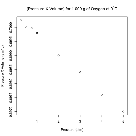
The right-most column is the product of pressure and temperature, and it is not constant.  However, are the differences between these values significant, or could it be due to some random variation (perhaps round-off error)?

Here is the scatter plot of the pressure-volume product with respect to pressure.

These points don’t look like they are on a horizontal line!  Let’s analyze these data using normal linear least-squares regression in R.

How to Calculate a Partial Correlation Coefficient in R: An Example with Oxidizing Ammonia to Make Nitric Acid

Introduction

Today, I will talk about the math behind calculating partial correlation and illustrate the computation in R.  The computation uses an example involving the oxidation of ammonia to make nitric acid, and this example comes from a built-in data set in R called stackloss.

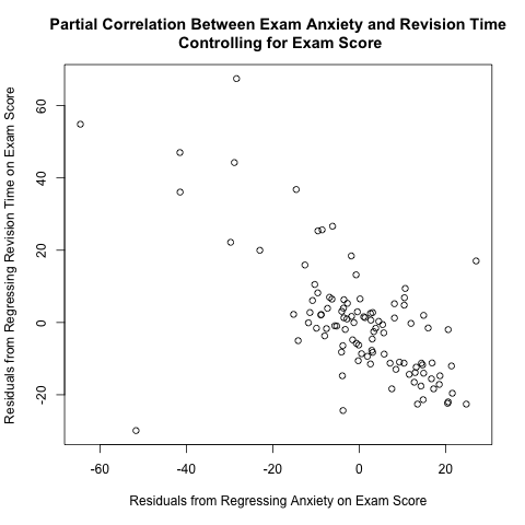
I read Pages 234-237 in Section 6.6 of “Discovering Statistics Using R” by Andy Field, Jeremy Miles, and Zoe Field to learn about partial correlation.  They used a data set called “Exam Anxiety.dat” available from their companion web site (look under “6 Correlation”) to illustrate this concept; they calculated the partial correlation coefficient between exam anxiety and revision time while controlling for exam score.  As I discuss further below, the plot between the 2 above residuals helps to illustrate the calculation of partial correlation coefficients.  This plot makes intuitive sense; if you take more time to study for an exam, you tend to have less exam anxiety, so there is a negative correlation between revision time and exam anxiety.

They used a function called pcor() in a package called “ggm”; however, I suspect that this package is no longer working properly, because it depends on a deprecated package called “RBGL” (i.e. “RBGL” is no longer available in CRAN).  See this discussion thread for further information.  Thus, I wrote my own R function to illustrate partial correlation.

Partial correlation is the correlation between 2 random variables while holding other variables constant.  To calculate the partial correlation between X and Y while holding Z constant (or controlling for the effect of Z, or averaging out Z),

How do Dew and Fog Form? Nature at Work with Temperature, Vapour Pressure, and Partial Pressure

In the early morning, especially here in Canada, I often see dew – water droplets formed by the condensation of water vapour on outside surfaces, like windows, car roofs, and leaves of trees.  I also sometimes see fog – water droplets or ice crystals that are suspended in air and often blocking visibility at great distances.  Have you ever wondered how they form?  It turns out that partial pressure, vapour pressure and temperature are the key phenomena at work.

Dew (by Staffan Enbom) and Fog (by Jon Zander)

Source: Wikimedia

Estimating the Decay Rate and the Half-Life of DDT in Trout – Applying Simple Linear Regression with Logarithmic Transformation

This blog post uses a function and a script written in R that were displayed in an earlier blog post.

Introduction

This is the second of a series of blog posts about simple linear regression; the first was written recently on some conceptual nuances and subtleties about this model.  In this blog post, I will use simple linear regression to analyze a data set with a logarithmic transformation and discuss how to make inferences on the regression coefficients and the means of the target on the original scale.  The data document the decay of dichlorodiphenyltrichloroethane (DDT) in trout in Lake Michigan; I found it on Page 49 in the book “Elements of Environmental Chemistry” by Ronald A. Hites.  Future posts will also be written on the chemical aspects of this topic, including the environmental chemistry of DDT and exponential decay in chemistry and, in particular, radiochemistry.

Dichlorodiphenyltrichloroethane (DDT)

Source: Wikimedia Commons

 

A serious student of statistics or a statistician re-learning the fundamentals like myself should always try to understand the math and the statistics behind a software’s built-in function rather than treating it like a black box.  This is especially worthwhile for a basic yet powerful tool like simple linear regression.  Thus, instead of simply using the lm() function in R, I will reproduce the calculations done by lm() with my own function and script (posted earlier on my blog) to obtain inferential statistics on the regression coefficients.  However, I will not write or explain the math behind the calculations; they are shown in my own function with very self-evident variable names, in case you are interested.  The calculations are arguably the most straightforward aspects of linear regression, and you can easily find the derivations and formulas on the web, in introductory or applied statistics textbooks, and in regression textbooks.

My Own R Function and Script for Simple Linear Regression – An Illustration with Exponential Decay of DDT in Trout

Here is the function that I wrote for doing simple linear regression, as alluded to in my blog post about simple linear regression on log-transformed data on the decay of DDT concentration in trout in Lake Michigan.  My goal was to replicate the 4 columns of the output from applying summary() to the output of lm().

To use this file and this script,

1) I saved this file as “simple linear regression.r”.

2) In the same folder, I saved a script called “DDT trout regression.r” that used this function to implement simple linear regression on the log-transformed DDT data.

3) I used setwd() to change the working directory to the folder containing the function and the script.

4) I made sure “DDT trout regression.r” used the source() function to call my user-defined function for simple linear regression.

5) I ran “DDT trout regression.r”.

Some Subtle and Nuanced Concepts about Simple Linear Regression

Introduction

This blog post will focus on some conceptual foundations of simple linear regression, a very common technique in statistics and a precursor for understanding multiple linear regression.  I will expose and clarify many nuances and subtleties that I did not fully absorb until my Master’s degree in statistics at the University of Toronto.

What is Simple Linear Regression?

Simple linear regression is a predictive model that uses a predictor variable (x) to predict a continuous target variable (Y).  It is a formal and rigorous way to express 2 fundamental components of a statistical predictive model.

1) For each value of x, there is a probability distribution of Y.

2) The means of the probability distributions for all values of Y vary with x in a systematic way.

Mathematically, the first component is reflected in a random error variable, and the second component is reflected in the constant that expresses the linear relationship between x and Y.  These two components add together to give the following mathematical model.

The last mathematical expression states that two different error terms are statistically independent.

Essentially, this model captures the tendency for Y to vary systematically with x.  The systematic part is the constant term, .  The tendency (rather than a direct relation) is reflected in the probability distribution of the error component.

Note that I capitalized the target Y because it is a random variable.  (It is a linear combination of the random error, so it is also a random variable.)  I used lower-case for the predictor because it is a constant in the model.

What are the Assumptions of Simple Linear Regression?

1) The predictor variable is a fixed constant with no random variation.  If you want to model the predictor as a random variable, use the errors-in-variables model (a.k.a. measurement errors model).

2) The target variable is a linear combination of the regression coefficients and the predictor.

3) The variance of the random error component is constant.  This assumptions is called homoscedasticity.

4) The random errors are independent of each other.

5) The regression coefficients are constants.  If you want to model the regression coefficients as random variables, use the random effects model.  If you want to include both fixed and random coefficients in your model, use the mixed effects model.  The documentation for PROX MIXED in SAS/STAT has a nice explanation of mixed effects model.  I also recommend the documentation for PROC GLM for more about the random effects model.

***6) The random errors are normally distributed with an expected value of 0 and a variance of .  As Assumption #3 states, this variance is constant for all .

***This last assumption is not needed for the least-squares estimation of the regression coefficients.  However, it is needed for conducting statistical inference for the regression coefficients, such as testing hypotheses and constructing confidence intervals.

Important Clarifications about the Terminology

Let me clarify some common confusion about the 2 key terms in the name “simple linear regression”.

– It is called “simple” because it uses only one predictor, whereas multiple linear regression uses multiple predictors.  While it is relatively simple to understand, and while it is a simple model compared to other predictive models, there are many concepts and nuances behind linear regression that still makes it difficult to understand for many people.  (I hope that this blog post will make it easier to understand this model!)

– It is called “linear” because the target variable is linear with respect to the parameters and  (the regression coefficients), not because it is linear with respect to the predictor; this is a very common misunderstanding, and I did not learn this until the second course in which I learned about linear regression.  This is more than just a naming custom; it implies that the regression coefficients can be estimated using linear algebra, which has many benefits that will be described in a later post.

Simple linear regression does assume that the target variable has a linear relationship with the predictor variable.  However, if it doesn’t, it can often be resolved – the predictor and/or the target can often be transformed to make the relationship linear.  If, however, the target variable cannot be written as a linear combination of the parameters  and , then the model is no longer linear regression, even if the target is linear with respect to the predictor.

How are the Regression Coefficients Estimated?

The regression coefficients are estimated by finding values of and that minimize the sum of the squares of the deviations from the regression line to the data.  My first linear regression textbook, “Applied Linear Statistical Models” by Kutner, Nachtsheim, Neter, and Li uses the letter “Q” to denote this quantity.  This is called the method of least squares.  The word “minimize” should trigger finding the global optimizers using differential calculus.

Differentiate Q with respect to and ; set the 2 derivatives to zero to get the normal equations.  The estimates are obtained by solving this system of 2 equations.

Why is the Least-Squares Method Used to Estimate the Regression Coefficients?

A natural question arises: Why minimize the sum of the squares of the errors?  Why not minimize some other measure of the distances from the regression line to the data, like the sum of the absolute values of the errors?

The answer lies within the Gauss-Markov theorem, which guarantees some very attractive properties for the least-squares estimators of the regression coefficients:

– these estimators are unbiased

– out of all linear unbiased estimators, the least-squares estimators have the minimum variance

Thus, the least-squares estimators are both accurate and very precise.

Note that the Gauss-Markov theorem holds without Assumption #6 above, which states that the errors have a normal distribution with an expected value of zero and a variance of .