Mathematical Statistics Lesson of the Day – Sufficient Statistics

*Update on 2014-11-06: Thanks to Christian Robert’s comment, I have removed the sample median as an example of a sufficient statistic.

Suppose that you collected data

in order to estimate a parameter .  Let be the probability density function (PDF)* for .

Let

be a statistic based on .  Let be the PDF for .

If the conditional PDF

is independent of , then is a sufficient statistic for .  In other words,

,

and does not appear in .

Intuitively, this means that contains everything you need to estimate , so knowing  (i.e. conditioning on ) is sufficient for estimating .

Often, the sufficient statistic for  is a summary statistic of , such as their

• sample mean
• sample median – removed thanks to comment by Christian Robert (Xi’an)
• sample minimum
• sample maximum

If such a summary statistic is sufficient for , then knowing this one statistic is just as useful as knowing all data for estimating .

*This above definition holds for discrete and continuous random variables.

Applied Statistics Lesson of the Day – The Coefficient of Variation

In my statistics classes, I learned to use the variance or the standard deviation to measure the variability or dispersion of a data set.  However, consider the following 2 hypothetical cases:

1. the standard deviation for the incomes of households in Canada is $2,000
2. the standard deviation for the incomes of the 5 major banks in Canada is $2,000

Even though this measure of dispersion has the same value for both sets of income data, $2,000 is a significant amount for a household, whereas $2,000 is not a lot of money for one of the “Big Five” banks.  Thus, the standard deviation alone does not give a fully accurate sense of the relative variability between the 2 data sets.  One way to overcome this limitation is to take the mean of the data sets into account.

A useful statistic for measuring the variability of a data set while scaling by the mean is the sample coefficient of variation:

where  is the sample standard deviation and is the sample mean.

Analogously, the coefficient of variation for a random variable is

where is the random variable’s standard deviation and is the random variable’s expected value.

The coefficient of variation is a very useful statistic that I, unfortunately, never learned in my introductory statistics classes.  I hope that all new statistics students get to learn this alternative measure of dispersion.

Mathematical and Applied Statistics Lesson of the Day – The Central Limit Theorem Can Apply to the Sum

The central limit theorem (CLT) is often stated in terms of the sample mean of independent and identically distributed random variables.  An often unnoticed or forgotten aspect of the CLT is its applicability to the sample sum of those variables.  Since , the sample size, is just a constant, it can be multiplied to to obtain .  For a sufficiently large , this new statistic still has an approximately normal distribution, just with a new expected value and a new variance.

Video Tutorial – Rolling 2 Dice: An Intuitive Explanation of The Central Limit Theorem

According to the central limit theorem, if

• random variables, , are independent and identically distributed,
• is sufficiently large,

then the distribution of their sample mean, , is approximately normal, and this approximation is better as increases.

One of the most remarkable aspects of the central limit theorem (CLT) is its validity for any parent distribution of .  In my new Youtube channel, you will find a video tutorial that provides an intuitive explanation of why this is true by considering a thought experiment of rolling 2 dice.  This video focuses on the intuition rather than the mathematics of the CLT.  In a later video, I will discuss the technical details of the CLT and how it applies to this example.

 

Mathematical and Applied Statistics Lesson of the Day – The Central Limit Theorem Applies to the Sample Mean

Having taught and tutored introductory statistics numerous times, I often hear students misinterpret the Central Limit Theorem by saying that, as the sample size gets bigger, the distribution of the data approaches a normal distribution.  This is not true.  If your data come from a non-normal distribution, their distribution stays the same regardless of the sample size.

Remember: The Central Limit Theorem says that, if is an independent and identically distributed sample of random variables, then the distribution of their sample mean is approximately normal, and this approximation gets better as the sample size gets bigger.

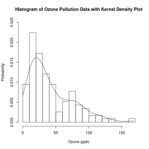
Exploratory Data Analysis: Combining Histograms and Density Plots to Examine the Distribution of the Ozone Pollution Data from New York in R

Introduction

This is a follow-up post to my recent introduction of histograms.  Previously, I presented the conceptual foundations of histograms and used a histogram to approximate the distribution of the “Ozone” data from the built-in data set “airquality” in R.  Today, I will examine this distribution in more detail by overlaying the histogram with parametric and non-parametric kernel density plots.  I will finally answer the question that I have asked (and hinted to answer) several times: Are the “Ozone” data normally distributed, or is another distribution more suitable?

Read the rest of this post to learn how to combine histograms with density curves like this above plot!

This is another post in my continuing series on exploratory data analysis (EDA).  Previous posts in this series on EDA include

• Descriptive statistics
• Box plots
• The conceptual foundations of kernel density estimation
• How to construct kernel density plots and rug plots in R
• Violin plots
• The conceptual foundations of empirical cumulative distribution functions (CDFs)
• 2 ways of plotting empirical CDFs in R
• The conceptual foundations of histograms