Applied Statistics Lesson of the Day – Polynomial Regression is Actually Just Linear Regression

Continuing from my previous Statistics Lesson of the Day on what “linear” really means in “linear regression”, I want to highlight a common example involving this nomenclature that can mislead non-statisticians.  Polynomial regression is a commonly used multiple regression technique; it models the systematic component of the regression model as a p\text{th}-order polynomial relationship between the response variable Y and the explanatory variable x.

Y = \beta_0 + \beta_1 x + \beta_2 x^2 + ... + \beta_p x^p + \varepsilon

However, this model is still a linear regression model, because the response variable is still a linear combination of the regression coefficients.  The regression coefficients would still be estimated using linear algebra through the method of least squares.

Remember: the “linear” in linear regression refers to the linearity between the response variable and the regression coefficients, NOT between the response variable and the explanatory variable(s).
Machine Learning Lesson of the Day – Estimating Coefficients in Linear Gaussian Basis Function Models

Recently, I introduced linear Gaussian basis function models as a suitable modelling technique for supervised learning problems that involve non-linear relationships between the target and the predictors.  Recall that linear basis function models are generalizations of linear regression that regress the target on functions of the predictors, rather than the predictors themselves.  In linear regression, the coefficients are estimated by the method of least squares.  Thus, it is natural that the estimation of the coefficients in linear Gaussian basis function models is an extension of the method of least squares.

The linear Gaussian basis function model is

Y = \Phi \beta + \varepsilon,

where \Phi_{ij} = \phi_j (x_i).  In other words, \Phi is the design matrix, and the element in row i and column j of this design matrix is the i\text{th} predictor being evaluated in the j\text{th} basis function.  (In this case, there is 1 predictor per datum.)

Applying the method of least squares, the coefficient vector, \beta, can be estimated by

\hat{\beta} = (\Phi^{T} \Phi)^{-1} \Phi^{T} Y.

Note that this looks like the least-squares estimator for the coefficient vector in linear regression, except that the design matrix is not X, but \Phi.

If you are not familiar with how \hat{\beta} was obtained, I encourage you to review least-squares estimation and the derivation of the estimator of the coefficient vector in linear regression.

How to Calculate a Partial Correlation Coefficient in R: An Example with Oxidizing Ammonia to Make Nitric Acid

Introduction

Today, I will talk about the math behind calculating partial correlation and illustrate the computation in R.  The computation uses an example involving the oxidation of ammonia to make nitric acid, and this example comes from a built-in data set in R called stackloss.

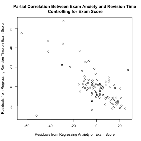
I read Pages 234-237 in Section 6.6 of “Discovering Statistics Using R” by Andy Field, Jeremy Miles, and Zoe Field to learn about partial correlation.  They used a data set called “Exam Anxiety.dat” available from their companion web site (look under “6 Correlation”) to illustrate this concept; they calculated the partial correlation coefficient between exam anxiety and revision time while controlling for exam score.  As I discuss further below, the plot between the 2 above residuals helps to illustrate the calculation of partial correlation coefficients.  This plot makes intuitive sense; if you take more time to study for an exam, you tend to have less exam anxiety, so there is a negative correlation between revision time and exam anxiety.

residuals plot anxiety and revision time controlling exam score

They used a function called pcor() in a package called “ggm”; however, I suspect that this package is no longer working properly, because it depends on a deprecated package called “RBGL” (i.e. “RBGL” is no longer available in CRAN).  See this discussion thread for further information.  Thus, I wrote my own R function to illustrate partial correlation.

Partial correlation is the correlation between 2 random variables while holding other variables constant.  To calculate the partial correlation between X and Y while holding Z constant (or controlling for the effect of Z, or averaging out Z),

Read more of this post

Presentation Slides – Overcoming Multicollinearity and Overfitting with Partial Least Squares Regression in JMP and SAS

My slides on partial least squares regression at the Toronto Area SAS Society (TASS) meeting on September 14, 2012, can be found here.

My Presentation on Partial Least Squares Regression

My first presentation to Toronto Area SAS Society (TASS) was delivered on September 14, 2012.  I introduced a supervised learning/predictive modelling technique called partial least squares (PLS) regression; I showed how normal linear least squares regression is often problematic when used with big data because of multicollinearity and overfitting, explained how partial least squares regression overcomes these limitations, and illustrated how to implement it in SAS and JMP.  I also highlighted the variable importance for projection (VIP) score that can be used to conduct variable selection with PLS regression; in particular, I documented its effectiveness as a technique for variable selection by comparing some key journal articles on this issue in academic literature.

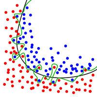
overfitting

The green line is an overfitted classifier.  Not only does it model the underlying trend, but it also models the noise (the random variation) at the boundary.  It separates the blue and the red dots perfectly for this data set, but it will classify very poorly on a new data set from the same population.

Source: Chabacano via Wikimedia
Read more of this post