Eric’s Enlightenment for Tuesday, May 26, 2015

1. Frances Woolley on the changing dynamics in the relationship between economists and the media in Canada over the past 8 years.
2. The unintended consequences of labour policies that are meant to be friendly for parents and families – a nice account of many examples by Claire Cain Miller.
3. FanGraphs explains batting average on balls in play (BABIP) in great detail.
4. How Neil Bartlett discovered compounds that contain noble gases.  (Yes – they can react!)  He began his research at the University of British Columbia in Vancouver (my hometown).  He also discovered a compound in which oxygen is a positively charged ion.  Very cool stuff!

When Does the Kinetic Theory of Gases Fail? Examining its Postulates with Assistance from Simple Linear Regression in R

Introduction

The Ideal Gas Law, , is a very simple yet useful relationship that describes the behaviours of many gases pretty well in many situations.  It is “Ideal” because it makes some assumptions about gas particles that make the math and the physics easy to work with; in fact, the simplicity that arises from these assumptions allows the Ideal Gas Law to be easily derived from the kinetic theory of gases.  However, there are situations in which those assumptions are not valid, and, hence, the Ideal Gas Law fails.

Boyle’s law is inherently a part of the Ideal Gas Law.  It states that, at a given temperature, the pressure of an ideal gas is inversely proportional to its volume.  Equivalently, it states the product of the pressure and the volume of an ideal gas is a constant at a given temperature.

An Example of The Failure of the Ideal Gas Law

This law is valid for many gases in many situations, but consider the following data on the pressure and volume of 1.000 g of oxygen at 0 degrees Celsius.  I found this data set in Chapter 5.2 of “General Chemistry” by Darrell Ebbing and Steven Gammon.

               Pressure (atm)      Volume (L)              Pressure X Volume (atm*L)
[1,]           0.25                2.8010                  0.700250
[2,]           0.50                1.4000                  0.700000
[3,]           0.75                0.9333                  0.699975
[4,]           1.00                0.6998                  0.699800
[5,]           2.00                0.3495                  0.699000
[6,]           3.00                0.2328                  0.698400
[7,]           4.00                0.1744                  0.697600
[8,]           5.00                0.1394                  0.697000

The right-most column is the product of pressure and temperature, and it is not constant.  However, are the differences between these values significant, or could it be due to some random variation (perhaps round-off error)?

Here is the scatter plot of the pressure-volume product with respect to pressure.

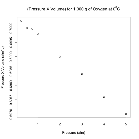
These points don’t look like they are on a horizontal line!  Let’s analyze these data using normal linear least-squares regression in R.

How to Calculate a Partial Correlation Coefficient in R: An Example with Oxidizing Ammonia to Make Nitric Acid

Introduction

Today, I will talk about the math behind calculating partial correlation and illustrate the computation in R.  The computation uses an example involving the oxidation of ammonia to make nitric acid, and this example comes from a built-in data set in R called stackloss.

I read Pages 234-237 in Section 6.6 of “Discovering Statistics Using R” by Andy Field, Jeremy Miles, and Zoe Field to learn about partial correlation.  They used a data set called “Exam Anxiety.dat” available from their companion web site (look under “6 Correlation”) to illustrate this concept; they calculated the partial correlation coefficient between exam anxiety and revision time while controlling for exam score.  As I discuss further below, the plot between the 2 above residuals helps to illustrate the calculation of partial correlation coefficients.  This plot makes intuitive sense; if you take more time to study for an exam, you tend to have less exam anxiety, so there is a negative correlation between revision time and exam anxiety.

They used a function called pcor() in a package called “ggm”; however, I suspect that this package is no longer working properly, because it depends on a deprecated package called “RBGL” (i.e. “RBGL” is no longer available in CRAN).  See this discussion thread for further information.  Thus, I wrote my own R function to illustrate partial correlation.

Partial correlation is the correlation between 2 random variables while holding other variables constant.  To calculate the partial correlation between X and Y while holding Z constant (or controlling for the effect of Z, or averaging out Z),