Mathematical Statistics Lesson of the Day – Complete Statistics

The set-up for today’s post mirrors my earlier Statistics Lesson of the Day on sufficient statistics.

Suppose that you collected data

in order to estimate a parameter .  Let be the probability density function (PDF)* for .

Let

be a statistic based on .

If

implies that

then  is said to be complete.  To deconstruct this esoteric mathematical statement,

1. let be a measurable function
2. if you want to use to form an unbiased estimator of the zero function,
3. and if the only such function is almost surely equal to the zero function,
4. then is a complete statistic.

I will discuss the intuition behind this bizarre definition in a later Statistics Lesson of the Day.

*This above definition holds for discrete and continuous random variables.

Exploratory Data Analysis: Conceptual Foundations of Empirical Cumulative Distribution Functions

Introduction

Continuing my recent series on exploratory data analysis (EDA), this post focuses on the conceptual foundations of empirical cumulative distribution functions (CDFs); in a separate post, I will show how to plot them in R.  (Previous posts in this series include descriptive statistics, box plots, kernel density estimation, and violin plots.)

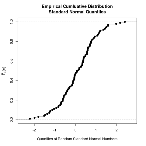
To give you a sense of what an empirical CDF looks like, here is an example created from 100 randomly generated numbers from the standard normal distribution.  The ecdf() function in R was used to generate this plot; the entire code is provided at the end of this post, but read my next post for more detail on how to generate plots of empirical CDFs in R.

Read to rest of this post to learn what an empirical CDF is and how to produce the above plot!