Video Tutorial – Rolling 2 Dice: An Intuitive Explanation of The Central Limit Theorem

According to the central limit theorem, if

• random variables, , are independent and identically distributed,
• is sufficiently large,

then the distribution of their sample mean, , is approximately normal, and this approximation is better as increases.

One of the most remarkable aspects of the central limit theorem (CLT) is its validity for any parent distribution of .  In my new Youtube channel, you will find a video tutorial that provides an intuitive explanation of why this is true by considering a thought experiment of rolling 2 dice.  This video focuses on the intuition rather than the mathematics of the CLT.  In a later video, I will discuss the technical details of the CLT and how it applies to this example.

 

Detecting Unfair Dice in Casinos with Bayes’ Theorem

Introduction

I saw an interesting problem that requires Bayes’ Theorem and some simple R programming while reading a bioinformatics textbook.  I will discuss the math behind solving this problem in detail, and I will illustrate some very useful plotting functions to generate a plot from R that visualizes the solution effectively.

The Problem

The following question is a slightly modified version of Exercise #1.2 on Page 8 in “Biological Sequence Analysis” by Durbin, Eddy, Krogh and Mitchison.

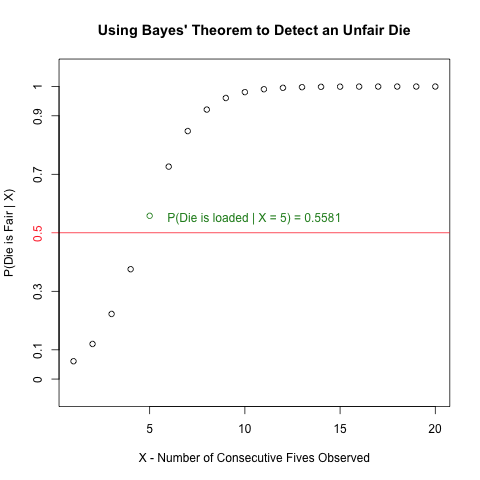
An occasionally dishonest casino uses 2 types of dice.  Of its dice, 97% are fair but 3% are unfair, and a “five” comes up 35% of the time for these unfair dice.  If you pick a die randomly and roll it, how many “fives”  in a row would you need to see before it was most likely that you had picked an unfair die?”

Read more to learn how to create the following plot and how it invokes Bayes’ Theorem to solve the above problem!